- adaboost 基本原理 B站5分钟机器学习
- 具体算法参考《统计学习方法》
思路
- 定义一个树桩——作为弱分类器
- 遍历数据集特征,根据最小分类误差率选择划分最优模型
- 计算弱分类器的权重、更新样本权重
- 线性组合弱分类器
第一步,定义树桩(弱分类器)
class DecisionStump():
    def __init__(self):
        self.polarity = 1                 # 分类结果(标识方向)
        # 1代表大于阈值判定为1,小于阈值判断为-1,-1反过来

        self.feature = None  # 使用的特征
        self.threshold = None        # 使用的阈值
        self.alpha = None             # 该分类器的权重
第二步,小例子
跟着《统计学习方法》8.1.3 adaboost的例子(只有一个特征)
梳理一下算法流程,做3个弱分类器的结合,可以完美拟合该数据
import numpy as np
import math

# 数据
x = np.array([0, 1, 2, 3, 4, 5, 6, 7, 8, 9])
y = np.array([1, 1, 1, -1, -1, -1, 1, 1, 1 ,-1])

# 初始化数据权值
w = [1 / len(x)] * len(x)

# 单个弱学习器的预测结果
def prediction(G, x):
    predictions = np.ones(np.shape(x))
    negative_idx = (G.polarity * x < G.polarity * G.threshold)
    predictions[negative_idx] = -1
    return predictions


######     第1个弱分类器     ######
G1 = DecisionStump()

# 1.找出分类误差率最低的阈值,保存为第一个弱分类器
error_ratio_old = 1.1
thresholds = np.arange(0.5, 9, 1)
for threshold in thresholds:
    polarity = 1
    res_error = (x <= threshold) * (y == polarity) + (x > threshold) * (y == -polarity)     # 分类错误
    error_ratio = np.dot(res_error, w)     # 误差率
    # 2.如果误差率大于0.5,说明方向反了
    if error_ratio > 0.5:
        polarity = -1
        error_ratio = 1 - error_ratio
    # 3.记录最小误差到第一个决策树桩
    if error_ratio < error_ratio_old:
        error_ratio_old = error_ratio
        G1.polarity = polarity
        G1.threshold = threshold
        G1.alpha = 1/2 * math.log((1 - error_ratio)/error_ratio)

# 4.对第一个弱分类器的测试,结果与书上一致
print("\n第一个弱分类器系数{}, 阈值{}, 方向{}".format(G1.alpha,G1.threshold,G1.polarity))
pred1 = prediction(G1, x)


######     第2个弱分类器     ######
G2 = DecisionStump()

# 1 .更新数据权值
def update_w(w, res, error_ratio):
    if res: return (0.5 * w / (1-error_ratio))
    else: return (0.5 * w / error_ratio)
print("\n更新数据权值:")
w1 = [update_w(w[i], pred1[i]==y[i], error_ratio_old) for i in range(len(w))]
w1

# 2.找出分类误差率最低的阈值,保存为第2个弱分类器
error_ratio_old = 1.1
for threshold in thresholds:
    polarity = 1
    res_error = (x <= threshold) * (y == polarity) + (x > threshold) * (y == -polarity)
    error_ratio = np.dot(res_error, w1)     # 误差率
    if error_ratio > 0.5:
        polarity = -1
        error_ratio = 1 - error_ratio
    if error_ratio < error_ratio_old:
        error_ratio_old = error_ratio
        G2.polarity = polarity
        G2.threshold = threshold
        G2.alpha = 1/2 * math.log((1 - error_ratio)/error_ratio)

pred2 = prediction(G2, x)
print("\n第二个弱分类器系数{}, 阈值{}, 方向{}".format(G2.alpha,G2.threshold,G2.polarity))


######     第3个弱分类器     ######
G3 = DecisionStump()
# 1 .更新数据权值
print("\n更新数据权值:")
w2 = [update_w(w1[i], pred2[i]==y[i], error_ratio_old) for i in range(len(w1))]
w2
# 2.找出分类误差率最低的阈值,保存为第2个弱分类器
error_ratio_old = 1.1
for threshold in thresholds:
    polarity = 1
    res_error = (x <= threshold) * (y == polarity) + (x > threshold) * (y == -polarity)
    error_ratio = np.dot(res_error, w2)     # 误差率
    if error_ratio > 0.5:
        polarity = -1
        error_ratio = 1 - error_ratio
    if error_ratio < error_ratio_old:
        error_ratio_old = error_ratio
        G3.polarity = polarity
        G3.threshold = threshold
        G3.alpha = 1/2 * math.log((1 - error_ratio)/error_ratio)

pred3 = prediction(G3, x)
print("\n第三个弱分类器系数{}, 阈值{}, 方向{}".format(G3.alpha,G3.threshold,G3.polarity))


######     结合两个弱分类器     ######
# 组合预测值
pred_y = np.ones(np.shape(x))
fx = pred1 * G1.alpha + pred2 * G2.alpha + pred3 * G3.alpha
negative_idx = (fx < 0)
pred_y[negative_idx] = -1
print("\n\n真实值:{}".format(y))
print("\nadaboost 预测值:{}".format(pred_y))
print("\n预测误差 = {}".format(np.mean(pred_y!=y)))
第一个弱分类器系数0.4236489301936017, 阈值2.5, 方向-1

更新数据权值:


[0.07142857142857144,
 0.07142857142857144,
 0.07142857142857144,
 0.07142857142857144,
 0.07142857142857144,
 0.07142857142857144,
 0.16666666666666666,
 0.16666666666666666,
 0.16666666666666666,
 0.07142857142857144]


第二个弱分类器系数0.64964149206513, 阈值8.5, 方向-1

更新数据权值:


[0.04545454545454547,
 0.04545454545454547,
 0.04545454545454547,
 0.1666666666666666,
 0.1666666666666666,
 0.1666666666666666,
 0.10606060606060608,
 0.10606060606060608,
 0.10606060606060608,
 0.04545454545454547]


第三个弱分类器系数0.7520386983881369, 阈值5.5, 方向1


真实值:[ 1  1  1 -1 -1 -1  1  1  1 -1]

adaboost 预测值:[ 1.  1.  1. -1. -1. -1.  1.  1.  1. -1.]

预测误差 = 0.0
第三步,多个特征的问题
核心:
- 遍历数据集特征和阈值,选择最小误差的特征和阈值,记录为该学习器
- 更新数据权值,重复上一步建立一个新的学习器
预测:
- 组合学习器计算最终预测值
沿用Dating数据集
import matplotlib.pyplot as plt
import pandas as pd

dating = pd.read_csv("Speed Dating Data.csv", encoding = "gbk")

## 提取变量——是否接受dec(因变量0-1)、好感度like、吸引力attr
dating = dating[['like','attr','dec']]
dating['dec'][dating["dec"]==0] = -1   # 处理为0-1变量
dating.head()

## 缺失问题
dating.isnull().sum(axis=0)  # 缺失比例
dating.dropna(axis = 0, how='any', thresh = None, subset = None, inplace=True)   # omit na值
print("去掉缺失之后总样本量{}".format(len(dating)))

## 分为训练集和测试集
sample = np.random.choice(range(len(dating)), int(len(dating)*0.8), replace= False).tolist()
dating_train = dating.iloc[sample, :]
dating_test = dating.iloc[[x for x in range(len(dating)) if x not in sample], :]
print("训练集样本量 = {}, 测试集样本量 = {}".format(len(dating_train),len(dating_test)))
| like | attr | dec | |
|---|---|---|---|
| 0 | 7.0 | 6.0 | 1 |
| 1 | 7.0 | 7.0 | 1 |
| 2 | 7.0 | 5.0 | 1 |
| 3 | 7.0 | 7.0 | 1 |
| 4 | 6.0 | 5.0 | 1 |
like    240
attr    202
dec       0
dtype: int64


去掉缺失之后总样本量8122
训练集样本量 = 6497, 测试集样本量 = 1625
逐个训练弱学习器
n_train = len(dating_train)
features = ['like','attr']
train_y = dating_train["dec"]


# 1.初始化权重1/N
w = np.full(n_train, (1/n_train))

# 2.逐个训练弱学习器
estimators = []   # 保存所有学习器
n_estimators = 6 # 准备造n_estimators个学习器
for _ in range(n_estimators):
    # 2.1 初始化
    G =  DecisionStump()
    error_ratio_min = 1.0
    # 2.2 遍历所有特征
    for feature in features:
        feature_values = dating_train[feature]
        unique_values = np.unique(feature_values)
        # 2.3 遍历该特征所有分类阈值
        for threshold in unique_values:
            polarity = 1  # 初始方向
            prediction = np.ones(n_train)
            prediction[feature_values < threshold] = -1
            error_ratio = sum(w[train_y != prediction])  # 误差率
            if error_ratio > 0.5:
                error_ratio = 1 - error_ratio
                polarity = -1

            if error_ratio < error_ratio_min:
                G.polarity = polarity
                G.threshold = threshold
                G.feature = feature
                G.alpha = 1/2 * math.log((1 - error_ratio)/error_ratio)
                error_ratio_min = error_ratio

    # 3.遍历结束之后
    # 3.1记录得到的学习器
    estimators.append(G)
    # 3.2 更新样本权值,以便下一个学习器的训练
    predictions = np.ones(n_train)
    negative_idx = (G.polarity * dating_train[G.feature] < G.polarity * G.threshold)
    predictions[negative_idx] = -1
    w *= np.exp(-G.alpha * train_y * predictions)
    w /= np.sum(w)

# 打印各个学习器的情况
for i in range(n_estimators):
    print("\n第{}个弱分类器\n特征{},系数{}, 阈值{}, 方向{}".format(i+1, \
                                              estimators[i].feature, estimators[i].alpha,estimators[i].threshold,estimators[i].polarity))
第1个弱分类器
特征like,系数0.5286878072409954, 阈值6.5, 方向1

第2个弱分类器
特征attr,系数0.2728648772469795, 阈值6.5, 方向1

第3个弱分类器
特征attr,系数0.1335036849107031, 阈值8.5, 方向1

第4个弱分类器
特征like,系数0.1361143472990432, 阈值6.5, 方向-1

第5个弱分类器
特征like,系数0.1783049598789307, 阈值5.5, 方向1

第6个弱分类器
特征like,系数0.10796016782025766, 阈值8.5, 方向1
组合预测
# 组合预测
fx = np.zeros(n_train)
for g in estimators:
    predictions = np.ones(n_train)
    negative_idx = (g.polarity * dating_train[g.feature] < g.polarity * g.threshold)
    predictions[negative_idx] = -1
    # 线性预测各个分类器的预测结果:
    fx += g.alpha * predictions


y_pred = np.ones(n_train)
index = (fx < 0)
y_pred[index] = -1
print("\n预测准确率 = {}".format(np.mean(y_pred==train_y)))

# 加载库画混淆矩阵
from sklearn.metrics import confusion_matrix
confusion_matrix(train_y, y_pred)
预测准确率 = 0.7434200400184701


array([[2742,  931],
       [ 736, 2088]])
第四步,定义class
class Adaboost():
    # 弱分类器
    def __init__(self, n_estimators = 5):
        self.n_estimators = n_estimators
        self.estimators = []

    # 拟合函数
    def fit(self, train_x, train_y, features):
        # 1.初始化权重1/N
        n_train = len(train_y)
        w = np.full(n_train, (1/n_train))

        # 2.逐个训练弱学习器
        for _ in range(self.n_estimators):
            # 2.1 初始化
            G =  DecisionStump()
            error_ratio_min = 1.0
            # 2.2 遍历所有特征
            for feature in features:
                feature_values = train_x[feature]
                unique_values = np.unique(feature_values)
                # 2.3 遍历该特征所有分类阈值
                for threshold in unique_values:
                    polarity = 1
                    prediction = np.ones(n_train)
                    prediction[feature_values < threshold] = -1
                    error_ratio = sum(w[train_y != prediction])
                    if error_ratio > 0.5:
                        error_ratio = 1 - error_ratio
                        polarity = -1
                    if error_ratio < error_ratio_min:
                        G.polarity = polarity
                        G.threshold = threshold
                        G.feature = feature
                        G.alpha = 1/2 * math.log((1 - error_ratio)/error_ratio)
                        error_ratio_min = error_ratio

            # 3.遍历结束之后
            # 3.1 记录得到的学习器
            self.estimators.append(G)
            # 3.2 更新样本权值,以便下一个学习器的训练
            predictions = np.ones(n_train)
            negative_idx = (G.polarity * train_x[G.feature] < G.polarity * G.threshold)
            predictions[negative_idx] = -1
            w *= np.exp( - G.alpha * train_y * predictions)
            w /= np.sum(w)


    # 组合预测函数
    def prediction(self, test):
        n = len(test)
        fx = np.zeros(n)
        for g in self.estimators:
            predictions = np.ones(n)
            negative_idx = (g.polarity * test[g.feature] < g.polarity * g.threshold)
            predictions[negative_idx] = -1
            fx += g.alpha * predictions  # 预测值

        # 根据预测值做出决策:
        y_pred = np.ones(n)
        index = (fx < 0)
        y_pred[index] = -1
        return fx, y_pred
不同学习器数量的预测结果:
myada1 = Adaboost(1)
myada1.fit(train_x = dating_train, train_y = dating_train["dec"], features = ['like','attr'])
test_fx, test_pred = myada1.prediction(dating_test)
print("\n包含1个学习器的adaboost,预测集上准确率 = {}".format(np.mean(test_pred==dating_test["dec"])))

myada2 = Adaboost(2)
myada2.fit(train_x = dating_train, train_y = dating_train["dec"], features = ['like','attr'])
test_fx, test_pred = myada2.prediction(dating_test)
print("\n包含7个学习器的adaboost,预测集上准确率 = {}".format(np.mean(test_pred==dating_test["dec"])))

myada15 = Adaboost(15)
myada15.fit(train_x = dating_train, train_y = dating_train["dec"], features = ['like','attr'])
test_fx, test_pred = myada15.prediction(dating_test)
print("\n包含15个学习器的adaboost,预测集上准确率 = {}".format(np.mean(test_pred==dating_test["dec"])))
包含1个学习器的adaboost,预测集上准确率 = 0.7341538461538462

包含2个学习器的adaboost,预测集上准确率 = 0.7569230769230769

包含15个学习器的adaboost,预测集上准确率 = 0.7796923076923077
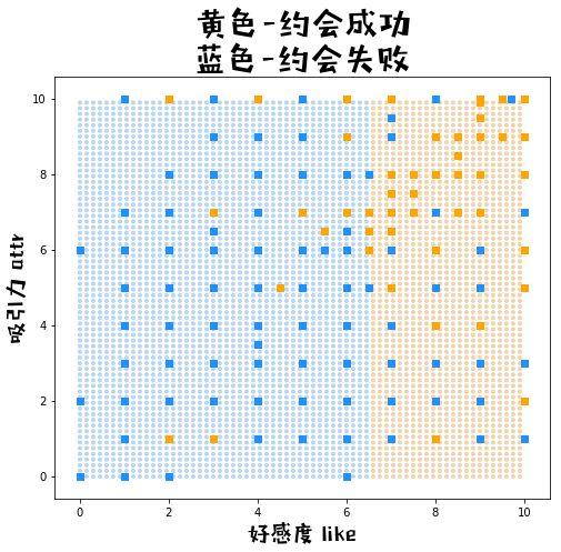
第五步,可视化分类界限
def plot_meshgrid(myada):
    # 1.生成网格点数据
    xx1, xx2 = np.meshgrid(np.arange(0, 10, 0.15), np.arange(0, 10, 0.15))   # 生成自变量的数据
    xx = pd.DataFrame({'like':xx1.ravel(),'attr':xx2.ravel()})                        # 拉直后合并为df
    yy_fx, yy_pred_ = myada.prediction(xx)
    yy_pred = np.array(yy_pred_).reshape(xx1.shape)                  # reshape为网格/矩阵

    # 2.画图
    fig = plt.figure(figsize=(8,7))   # 创建一张8*6的画布
    # 2.1背景网格点
    color = ["#e2a653" if c==1 else "#6cabe6" for c in yy_pred_]
    plt.scatter(xx1, xx2, c = color, alpha = 0.4, marker= ".")

    # 2.2原始数据的点
    color = ["orange" if c==1 else "dodgerblue" for c in dating_train['dec']]
    plt.scatter(dating_train['like'],dating_train['attr'], c=color, marker= "s")

    # 3.图例
    plt.title('黄色-约会成功\n蓝色-约会失败', fontproperties=prop, fontsize=30)
    plt.xlabel("好感度 like", fontproperties=prop, fontsize=20)
    plt.ylabel("吸引力 attr", fontproperties=prop, fontsize=20)
plot_meshgrid(myada1)
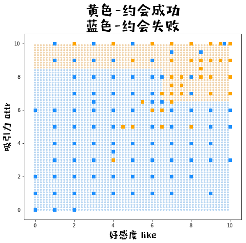
plot_meshgrid(myada2)
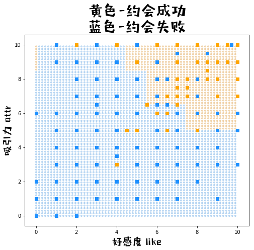
plot_meshgrid(myada15)