- 处理有解/x'x可逆的情况——非常简单的矩阵运算
- 补充上岭回归的惩罚参数a——也是简单的矩阵运算,也可以用梯度下降
- 交叉验证——计算平均预测误差 RMSE 在多次中的平均值
关键在于包装为成一个尽可能完整的class
Ridge 的封装——类
想要实现的功能:
- 划分训练和测试集
- 梯度下降迭代估计参数
- 绘制迭代cost收敛图
- 计算预测值
- 计算预测rmse
- 交叉验证的平均rmse
读入& 处理数据 & 提取变量
import os
import numpy as np
import matplotlib.pyplot as plt
import pandas as pd
#  1.读入数据
os.chdir("/Users/mac/Desktop/快乐研一/python/data")
gaokao = pd.read_csv("高考待预处理.csv")
gaokao.head()
data = gaokao.iloc[:, [2, 3, 11, 4]]
data_x = data.drop(["分数线"], axis=1)  # # 提取自变量——重点学科、博士点、是否为综合类大学
data_y = data[['分数线']]  # 因变量——分数线
# 2.标准化
def biaozhunhua(x):
    return (x-x.mean())/x.std()
data_y = data_y.apply(biaozhunhua)
data_x[["重点学科","博士点"]] = data_x[["重点学科","博士点"]].apply(biaozhunhua)
| 大学名称 | 类型 | 重点学科 | 博士点 | 分数线 | type_农业 | type_医药 | type_工科 | type_师范 | type_林业 | type_民族 | type_综合 | type_财经 | |
|---|---|---|---|---|---|---|---|---|---|---|---|---|---|
| 0 | 北京大学 | 综合 | 81.0 | 201.0 | 694.0 | 0 | 0 | 0 | 0 | 0 | 0 | 1 | 0 |
| 3 | 复旦大学 | 综合 | 30.0 | 178.0 | 687.0 | 0 | 0 | 0 | 0 | 0 | 0 | 1 | 0 |
| 4 | 清华大学 | 综合 | 37.0 | 253.0 | 686.0 | 0 | 0 | 0 | 0 | 0 | 0 | 1 | 0 |
| 5 | 上海交通大学 | 综合 | 9.0 | 78.0 | 664.0 | 0 | 0 | 0 | 0 | 0 | 0 | 1 | 0 |
| 7 | 南京大学 | 综合 | 21.0 | 44.0 | 662.0 | 0 | 0 | 0 | 0 | 0 | 0 | 1 | 0 |
具体实现(梯度下降)
- 岭回归也可以通过矩阵求逆直接计算
- 这里当做优化问题来做——梯度下降法
class Ridge():
def __init__(self):
self.w = None
self.b = None
self.costlist = None
self.epochs = None
# 1.获得参数估计值
def getParam(self):
print("\nW: {}\nb: {}".format(np.round(self.w,3), np.round(self.b,3)))
return self.w, self.b
# 2.计算梯度
def l2_loss(self, X, y, w, b, alpha = 0):
num_train = X.shape[0]
num_feature = X.shape[1]
y_hat = np.dot(X, w) + b
cost = np.sum((y_hat-y)**2)/num_train + alpha*(np.sum(np.square(w)))
dw = np.dot(X.T, (y_hat-y)) /num_train + 2*alpha*w
db = np.sum((y_hat-y)) /num_train
return dw, db, cost
# 3.迭代估计
def fit(self, data_x, data_y, learning_rate=0.05, epochs=1000, alpha=0, ifprint = False):
'''
输入:X、y、学习率、迭代次数、惩罚系数
输出:估计参数、cost(list)
'''
self.w = np.zeros((data_x.shape[1],1))
self.b = 0
self.costlist = []
self.epochs = epochs
for i in range(epochs):
dw, db, cost_tmp = self.l2_loss(data_x, data_y, self.w, self.b, alpha = alpha) # 计算梯度
self.w = self.w - learning_rate * dw # 更新参数
self.b = self.b - learning_rate * db
self.b = self.b.tolist()
self.costlist.append(cost_tmp) # 记录下cost函数的递减过程
if (ifprint==True) and (i % 100 == 0): # 打印训练过程
print("迭代次数:%d, cost=%f" % (i+1, cost_tmp))
if ifprint==True:
print("%d次迭代结束!最终训练集上cost:%f" % (i+1, cost_tmp))
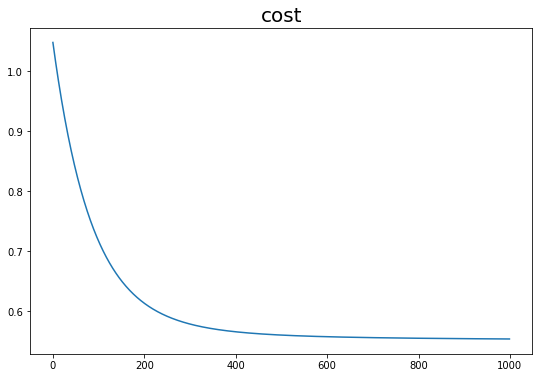
# 4.绘制cost收敛
def plot_cost(self):
fig = plt.figure(figsize=(9,6))
plt.plot(range(self.epochs), self.costlist)
plt.title("cost", fontsize=20)
plt.show()
plt.close()
#5. 计算rmse:
def rmse(self, test_y, test_pred):
x = np.squeeze(np.array(test_y))-test_pred
return np.sqrt(np.squeeze(np.dot((x).T,(x)))/len(x))
# 6.计算预测值
def prediction(self, test_x):
yhat_l2 = np.squeeze(np.dot(test_x, self.w) + self.b)
return yhat_l2
# 7.# 划分训练集和测试集
def sample(self, data_x, data_y, percentage=0.8):
sample = np.random.choice(range(len(data_y)), int(len(data_y) * percentage), replace= False).tolist()
train_x = data_x.iloc[sample, :]
test_x = data_x.iloc[[x for x in range(len(data_y)) if x not in sample], :]
train_y = data_y.iloc[sample, :]
test_y = data_y.iloc[[x for x in range(len(data_y)) if x not in sample], :]
print("训练集样本量:{}测试集样本量:{}".format(len(train_y),len(test_y)))
return train_x, train_y, test_x, test_y
### 测试 ridge 函数类
# 1.初始化
model = Ridge()
# 2.分割测试和训练
train_x, train_y, test_x, test_y = model.sample(data_x, data_y, percentage=0.7)
# 3.训练model
model.fit(train_x, train_y, learning_rate=0.003, epochs=1000, alpha=0.1, ifprint = True)
# 4.获取参数估计值
w, b = model.getParam()
# 5.绘制训练过程中的cost收敛过程
model.plot_cost()
# 6. 预测
test_pred = model.prediction(test_x)
# 7.计算预测rmse
rmse_l2 = model.rmse(test_y, test_pred)
print("\n 岭回归(惩罚系数0.1\n预测集上rmse={}".format(rmse_l2))
训练集样本量:89测试集样本量:39
迭代次数:1,  cost=1.048072
迭代次数:101,  cost=0.716701
迭代次数:201,  cost=0.613186
迭代次数:301,  cost=0.578509
迭代次数:401,  cost=0.565609
迭代次数:501,  cost=0.560109
迭代次数:601,  cost=0.557384
迭代次数:701,  cost=0.555831
迭代次数:801,  cost=0.554838
迭代次数:901,  cost=0.554142
1000次迭代结束!最终训练集上cost:0.553627

W: [[ 0.321]
 [ 0.364]
 [-0.05 ]]
b: [-0.052]
 岭回归(惩罚系数0.1
预测集上rmse=0.7781370066362491
定义函数——普通最小二乘(矩阵求逆)
$rmse = \frac{(X\beta -y)'(X\beta -y)}{n} $
##### 正式定义函数——OLS
def my_OLS(data_x, data_y):

    #######    1.构造数据    ######
    #  在第一列插入1
    col_name = data_x.columns.tolist()
    col_name.insert(0, 'x0')
    data_x = data_x.reindex(columns = col_name)
    data_x['x0'] = [1] * data_x.shape[0]

    #######    2.计算OLS估计量    ######
    xTx = np.dot(data_x.T, data_x)   # x'x
    xTx_I = np.matrix(xTx).I            # (x'x)的逆
    beta = np.dot(np.dot(xTx_I, data_x.T), data_y)
    beta = np.squeeze(np.array(beta))

    #######    3.输出    ######
    yhat = np.dot(data_x, beta)
    return yhat, beta

# 测试
# train_x, train_y, test_x, test_y
yhat_ols, beta_ols = my_OLS(train_x, train_y)
yhat_ols = np.dot(beta_ols[1:len(beta_ols)], test_x.T) + beta_ols[0]
rmse_ols = model.rmse(test_y, yhat_ols)   # 普通最小二乘rmse
print("普通最小二乘法参数:{} \n 预测集上rmse={}".format(np.round(beta_ols,3),np.round(rmse_ols,3)))
普通最小二乘法参数:[ 0.034  0.344  0.479 -0.029]
 预测集上rmse=0.793