knn算法实现
思路
-
定义函数——计算训练集各数据与给出实例的距离
-
定义函数——投票规则
根据最近的k个训练数据——投票得到新实例的类别 -
定义函数——交叉验证选择最佳k值
一般可以先根据样本量来选择k值范围,最后交叉验证取预测率最高的k值
-
可视化不同k带来的影响
数据预处理
和之前一样,直接复制
import os
import numpy as np
import matplotlib.pyplot as plt
import pandas as pd

## 将代码块运行结果全部输出,而不是只输出最后的,适用于全文
from IPython.core.interactiveshell import InteractiveShell
InteractiveShell.ast_node_interactivity = "all"
## 不显示warnings
import warnings
warnings.filterwarnings("ignore")

# font_manager函数,用于指定中文字体样式、大小
import matplotlib.font_manager as mfm
font_path = r"/Users/mac/Library/Fonts/字体管家方萌简(非商业使用)v1.1.ttf"
prop = mfm.FontProperties(fname = font_path)

## 读入数据
os.chdir("/Users/mac/Desktop/快乐研一/python/机器学习python实现")
dating = pd.read_csv("Speed Dating Data.csv", encoding = "gbk")

## 提取变量——是否接受dec(因变量0-1)、好感度like、吸引力attr
dating = dating[['like','attr','dec']]
dating.head()

## 缺失问题
dating.isnull().sum(axis=0)  # 缺失比例
dating.dropna(axis = 0, how='any', thresh = None, subset = None, inplace=True)   # omit na值
print("去掉缺失之后总样本量{}".format(len(dating)))

## 分为训练集和测试集
sample = np.random.choice(range(len(dating)), int(len(dating)*0.8), replace= False).tolist()
dating_train = dating.iloc[sample, :]
dating_test = dating.iloc[[x for x in range(len(dating)) if x not in sample], :]
print("训练集样本量 = {}, 测试集样本量 = {}".format(len(dating_train),len(dating_test)))
去掉缺失之后总样本量8122
训练集样本量 = 6497, 测试集样本量 = 1625
定义函数——计算训练集与给出实例的距离
- 第i和第j样本的L2距离:
- 输入:训练集用矩阵输入X (n,p),测试集用向量输入x(1,p)
- 输出:距离向量dist(1,n) 表示每个训练集样本点与实例的距离
def L2_Distance(example, train):
    dist = train-example              # 训练集的每一行都减掉实例
    dist_ = np.square(dist)           # 每个元素求平方
    l2dist = np.sqrt(dist_.sum(axis = 1))      # 按行相加后开根号
    return l2dist.tolist()

example = dating_test.iloc[0,:].tolist()
dating_dist = L2_Distance(example[:2], dating_train[['like','attr']])
np.max(dating_dist),np.min(dating_dist)
(9.219544457292887, 0.0)
定义函数——投票给出实例预测类别
def prediction(example, train, ylabel, k):
    '''
    输入:example(没有类别变量),train,ylabel(标识train类别变量),k(用k个投票)
    输出:投票结果
    '''
    # 提取自变量和因变量
    xlabel = [x for x in train.columns.tolist() if x!=ylabel]
    train_x = train[xlabel]
    train_y = np.array(train[ylabel])
    # 取出k个最近样本点的类别结果
    dist = L2_Distance(example, train_x)   # 计算distance
    labels = train_y[np.argsort(dist)]  # 距离按大小排序
    labels_k = labels[0:k]   # 提取k个最近的
    # 计算投票结果
    results = labels_k.sum()/k
    if results>=0.5:
        return 1
    else:
        return 0


# 测试1
example = dating_test.iloc[0, ]
example['like'] = 9.0; example['attr'] = 10.0;
print("测试数据1:\n{},预测结果{}\n".format(example[:2], prediction(example[:2], dating_train,"dec", 30)))

# 测试2
example['like'] = 5.0; example['attr'] = 4.0;
print("测试数据2:\n{},预测结果{}\n".format(example[:2], prediction(example[:2], dating_train,"dec", 30)))
测试数据1:
like     9.0
attr    10.0
Name: 0, dtype: float64,预测结果1

测试数据2:
like    5.0
attr    4.0
Name: 0, dtype: float64,预测结果0
选取最优k值
- 交叉验证计算验证集上——平均预测准确率
- 遍历k值可能取值选择预测最好的
def cv_accuracy(train, ylabel, klist, num_fold = 5):
    # 划分训练、验证集
    data_split = np.array_split(train, num_fold)
    xlabel = [x for x in train.columns.tolist() if x!=ylabel]
    accuracy_k = []
    for k in klist:
        mean_accuracy = []
        for fold in range(num_fold):      # n折交叉验证
            # 处理数据格式
            data_dev = data_split[fold]   # 一份作为验证集
            data_dev_x = data_dev[xlabel] # 去掉因变量
            data_train = np.concatenate(data_split[:fold] + data_split[fold+1:])   # 其他合并为训练集
            data_train = pd.DataFrame(data_train)
            data_train.columns = train.columns
            data_dev_pred = []
            # 计算结果
            for i in range(data_dev_x.shape[0]):
                predi = prediction(data_dev_x.iloc[i,:], data_train, ylabel, k)
                data_dev_pred.append(predi)
            print("进行到k = {} 时的第{}次交叉验证".format(k, fold+1))
            accuracy = (data_dev_pred==data_dev[ylabel]).mean()
            mean_accuracy.append(accuracy)
        print("k = {}, 验证集平均预测正确率 = {}".format(k, np.mean(mean_accuracy)))
        accuracy_k.append(np.mean(mean_accuracy))
    return accuracy_k

# 测试:
cv_accuracy(dating_train, 'dec', [1, 5, 10, 30, 50, 100, 300, 500, 3000], num_fold = 5)
进行到k = 1 时的第1次交叉验证
进行到k = 1 时的第2次交叉验证
进行到k = 1 时的第3次交叉验证
进行到k = 1 时的第4次交叉验证
进行到k = 1 时的第5次交叉验证
k = 1, 验证集平均预测正确率 = 0.6761536092852489
进行到k = 5 时的第1次交叉验证
进行到k = 5 时的第2次交叉验证
进行到k = 5 时的第3次交叉验证
进行到k = 5 时的第4次交叉验证
进行到k = 5 时的第5次交叉验证
k = 5, 验证集平均预测正确率 = 0.7180248712027003
进行到k = 10 时的第1次交叉验证
进行到k = 10 时的第2次交叉验证
进行到k = 10 时的第3次交叉验证
进行到k = 10 时的第4次交叉验证
进行到k = 10 时的第5次交叉验证
k = 10, 验证集平均预测正确率 = 0.7392647598744595
进行到k = 30 时的第1次交叉验证
进行到k = 30 时的第2次交叉验证
进行到k = 30 时的第3次交叉验证
进行到k = 30 时的第4次交叉验证
进行到k = 30 时的第5次交叉验证
k = 30, 验证集平均预测正确率 = 0.7503458281518328
进行到k = 50 时的第1次交叉验证
进行到k = 50 时的第2次交叉验证
进行到k = 50 时的第3次交叉验证
进行到k = 50 时的第4次交叉验证
进行到k = 50 时的第5次交叉验证
k = 50, 验证集平均预测正确率 = 0.759887724284953
进行到k = 100 时的第1次交叉验证
进行到k = 100 时的第2次交叉验证
进行到k = 100 时的第3次交叉验证
进行到k = 100 时的第4次交叉验证
进行到k = 100 时的第5次交叉验证
k = 100, 验证集平均预测正确率 = 0.7578870136791614
进行到k = 300 时的第1次交叉验证
进行到k = 300 时的第2次交叉验证
进行到k = 300 时的第3次交叉验证
进行到k = 300 时的第4次交叉验证
进行到k = 300 时的第5次交叉验证
k = 300, 验证集平均预测正确率 = 0.7605033457689346
进行到k = 500 时的第1次交叉验证
进行到k = 500 时的第2次交叉验证
进行到k = 500 时的第3次交叉验证
进行到k = 500 时的第4次交叉验证
进行到k = 500 时的第5次交叉验证
k = 500, 验证集平均预测正确率 = 0.7632748267898384
进行到k = 3000 时的第1次交叉验证
进行到k = 3000 时的第2次交叉验证
进行到k = 3000 时的第3次交叉验证
进行到k = 3000 时的第4次交叉验证
进行到k = 3000 时的第5次交叉验证
k = 3000, 验证集平均预测正确率 = 0.7601971931071239


[0.6761536092852489,
 0.7180248712027003,
 0.7392647598744595,
 0.7503458281518328,
 0.759887724284953,
 0.7578870136791614,
 0.7605033457689346,
 0.7632748267898384,
 0.7601971931071239]
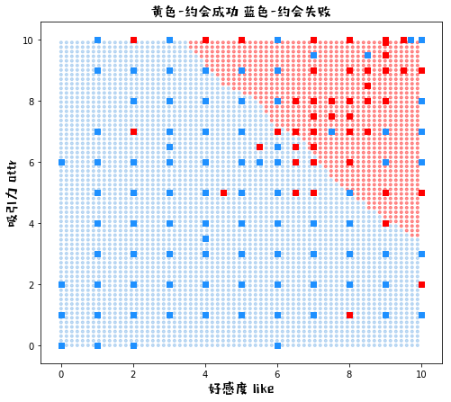
可视化不同k下的结果
def plot_knn_k(k):
    # 1.生成网格点数据
    xx1, xx2 = np.meshgrid(np.arange(0, 10, 0.15), np.arange(0, 10, 0.15))   # 生成自变量的数据
    xx = pd.DataFrame({'like':xx1.ravel(),'attr':xx2.ravel()})                         # 拉直后合并为df
    yy_pred_ = []   # 预测
    for i in range(len(xx)):
        yy_pred_.append(prediction(xx.iloc[i,], dating_train, "dec", k))
    yy_pred = np.array(yy_pred_).reshape(xx1.shape)                  # reshape为网格/矩阵

    # 2.画图
    fig = plt.figure(figsize=(8,7))   # 创建一张8*6的画布
    # 2.1背景网格点
    color = ["red" if c==1 else "#6cabe6" for c in yy_pred_]
    plt.scatter(xx1, xx2, c = color, alpha = 0.4, marker= ".")

    # 2.2原始数据的点
    color = ["red" if c==1 else "dodgerblue" for c in dating['dec']]
    plt.scatter(dating['like'],dating['attr'], c=color, marker= "s")

    # 3.图例
    print("\nK = {}".format(k))
    plt.title('黄色-约会成功 蓝色-约会失败', fontproperties = prop, fontsize = 15)
    plt.xlabel("好感度 like", fontproperties = prop, fontsize = 15)
    plt.ylabel("吸引力 attr", fontproperties = prop, fontsize = 15)
plot_knn_k(k=1)
K = 1
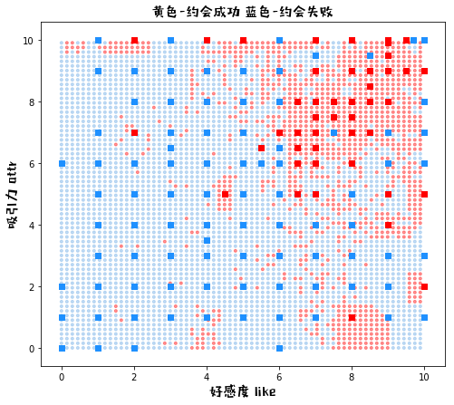
plot_knn_k(k=50)
K = 50
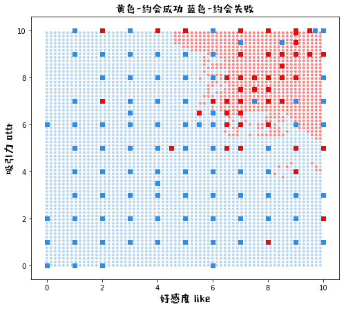
plot_knn_k(k=500)
K = 500
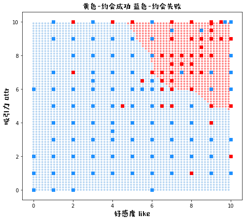
plot_knn_k(k=3000)
K = 3000